Analysing GITT data#
PyProBE includes built-in analysis methods for pulsing experiments, which this example will demonstrate.
First import the required libraries and data:
%%capture
%pip install matplotlib
import matplotlib.pyplot as plt

import pyprobe

%matplotlib inline
info_dictionary = {
    "Name": "Sample cell",
    "Chemistry": "NMC622",
    "Nominal Capacity [Ah]": 0.04,
    "Cycler number": 1,
    "Channel number": 1,
}
data_directory = "../../../tests/sample_data/neware"

# Create a cell object
cell = pyprobe.Cell(info=info_dictionary)
cell.import_from_cycler(
    procedure_name="Sample",
    cycler="neware",
    input_data_path=data_directory + "/sample_data_neware.xlsx",
)
print(cell.procedure["Sample"].experiment_names)
['Initial Charge', 'Break-in Cycles', 'Discharge Pulses']
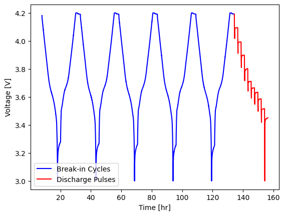
We will plot the Break-in Cycles and Discharge Pulses:
fig, ax = plt.subplots()
cell.procedure["Sample"].experiment("Break-in Cycles").plot(
    x="Time [hr]",
    y="Voltage [V]",
    ax=ax,
    label="Break-in Cycles",
    color="blue",
)
cell.procedure["Sample"].experiment("Discharge Pulses").plot(
    x="Time [hr]",
    y="Voltage [V]",
    ax=ax,
    label="Discharge Pulses",
    color="red",
)
ax.set_ylabel("Voltage [V]")
Text(0, 0.5, 'Voltage [V]')
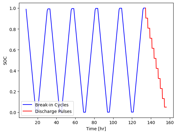
State-of-charge is a useful metric when working with battery data, however it must be carefully defined. PyProBE doesn’t automatically calculate a value for cell SOC until instructed to by the user for this reason.
To add an SOC column to the data, we call set_soc() on the procedure. We are going to provide an argument to reference_charge. This will be the final charge of the break-in cycles. This argument instructs PyProBE that the final data point of this charge is our 100% SOC reference.
reference_charge = cell.procedure["Sample"].experiment("Break-in Cycles").charge(-1)
cell.procedure["Sample"].set_soc(reference_charge=reference_charge)

fig, ax = plt.subplots()
cell.procedure["Sample"].experiment("Break-in Cycles").plot(
    x="Time [hr]",
    y="SOC",
    ax=ax,
    label="Break-in Cycles",
    color="blue",
)
cell.procedure["Sample"].experiment("Discharge Pulses").plot(
    x="Time [hr]",
    y="SOC",
    ax=ax,
    label="Discharge Pulses",
    color="red",
)
ax.set_ylabel("SOC")
plt.legend(loc="lower left")
<matplotlib.legend.Legend at 0x77c614504b00>
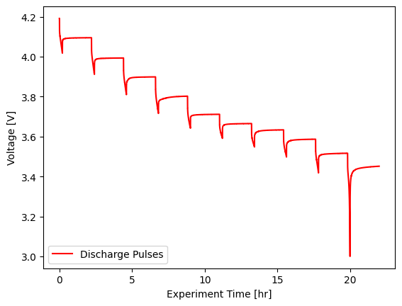
Then we’ll filter to only the pulsing experiment:
pulsing_experiment = cell.procedure["Sample"].experiment("Discharge Pulses")

fig, ax = plt.subplots()
pulsing_experiment.plot(
    x="Experiment Time [hr]",
    y="Voltage [V]",
    ax=ax,
    label="Discharge Pulses",
    color="red",
)
ax.set_ylabel("Voltage [V]")
plt.legend(loc="lower left")
<matplotlib.legend.Legend at 0x77c613b46330>
And then create our pulsing analysis object.
from pyprobe.analysis import pulsing

pulse_object = pulsing.Pulsing(input_data=pulsing_experiment)
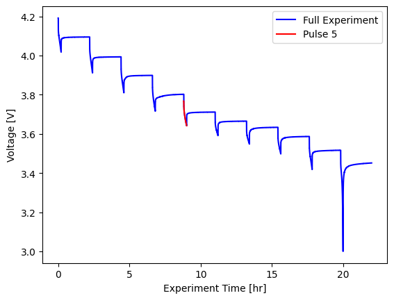
With the pulsing object we can separate out individual pulses:
fig, ax = plt.subplots()
pulse_object.input_data.plot(
    x="Experiment Time [hr]",
    y="Voltage [V]",
    label="Full Experiment",
    color="blue",
    ax=ax,
)
pulse_object.pulse(4).plot(
    x="Experiment Time [hr]",
    y="Voltage [V]",
    label="Pulse 5",
    color="red",
    ax=ax,
)
ax.set_ylabel("Voltage [V]")
Text(0, 0.5, 'Voltage [V]')
We can also extract key parameters from the pulsing experiment, with the get_resistances() method.
pulse_resistances = pulsing.get_resistances(input_data=pulsing_experiment)
print(pulse_resistances.data)
shape: (10, 5)
┌──────────────┬───────────────┬──────────┬─────────┬───────────┐
│ Pulse Number ┆ Capacity [Ah] ┆ SOC      ┆ OCV [V] ┆ R0 [Ohms] │
│ ---          ┆ ---           ┆ ---      ┆ ---     ┆ ---       │
│ u32          ┆ f64           ┆ f64      ┆ f64     ┆ f64       │
╞══════════════╪═══════════════╪══════════╪═════════╪═══════════╡
│ 1            ┆ 0.062214      ┆ 1.0      ┆ 4.1919  ┆ 1.805578  │
│ 2            ┆ 0.058214      ┆ 0.903497 ┆ 4.0949  ┆ 1.835632  │
│ 3            ┆ 0.054213      ┆ 0.806994 ┆ 3.9934  ┆ 1.775612  │
│ 4            ┆ 0.050213      ┆ 0.710493 ┆ 3.8987  ┆ 1.750596  │
│ 5            ┆ 0.046213      ┆ 0.613991 ┆ 3.8022  ┆ 1.725532  │
│ 6            ┆ 0.042212      ┆ 0.517489 ┆ 3.7114  ┆ 1.705558  │
│ 7            ┆ 0.038212      ┆ 0.420988 ┆ 3.665   ┆ 1.705622  │
│ 8            ┆ 0.034212      ┆ 0.324487 ┆ 3.6334  ┆ 1.735555  │
│ 9            ┆ 0.030212      ┆ 0.227986 ┆ 3.5866  ┆ 1.795638  │
│ 10           ┆ 0.026211      ┆ 0.131485 ┆ 3.5164  ┆ 1.900663  │
└──────────────┴───────────────┴──────────┴─────────┴───────────┘
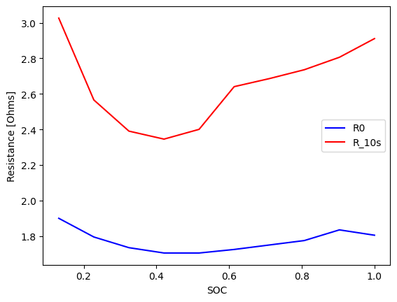
The get_resistances() method can take an argument of a list of times at which to evaluate the resistance after the pulse, for instance at 10s after the pulse:
pulse_resistances = pulsing.get_resistances(input_data=pulsing_experiment, r_times=[10])
print(pulse_resistances.data)
shape: (10, 6)
┌──────────────┬───────────────┬──────────┬─────────┬───────────┬──────────────┐
│ Pulse Number ┆ Capacity [Ah] ┆ SOC      ┆ OCV [V] ┆ R0 [Ohms] ┆ R_10s [Ohms] │
│ ---          ┆ ---           ┆ ---      ┆ ---     ┆ ---       ┆ ---          │
│ u32          ┆ f64           ┆ f64      ┆ f64     ┆ f64       ┆ f64          │
╞══════════════╪═══════════════╪══════════╪═════════╪═══════════╪══════════════╡
│ 1            ┆ 0.062214      ┆ 1.0      ┆ 4.1919  ┆ 1.805578  ┆ 2.910931     │
│ 2            ┆ 0.058214      ┆ 0.903497 ┆ 4.0949  ┆ 1.835632  ┆ 2.805967     │
│ 3            ┆ 0.054213      ┆ 0.806994 ┆ 3.9934  ┆ 1.775612  ┆ 2.735943     │
│ 4            ┆ 0.050213      ┆ 0.710493 ┆ 3.8987  ┆ 1.750596  ┆ 2.685915     │
│ 5            ┆ 0.046213      ┆ 0.613991 ┆ 3.8022  ┆ 1.725532  ┆ 2.640815     │
│ 6            ┆ 0.042212      ┆ 0.517489 ┆ 3.7114  ┆ 1.705558  ┆ 2.400785     │
│ 7            ┆ 0.038212      ┆ 0.420988 ┆ 3.665   ┆ 1.705622  ┆ 2.345855     │
│ 8            ┆ 0.034212      ┆ 0.324487 ┆ 3.6334  ┆ 1.735555  ┆ 2.390765     │
│ 9            ┆ 0.030212      ┆ 0.227986 ┆ 3.5866  ┆ 1.795638  ┆ 2.565912     │
│ 10           ┆ 0.026211      ┆ 0.131485 ┆ 3.5164  ┆ 1.900663  ┆ 3.026056     │
└──────────────┴───────────────┴──────────┴─────────┴───────────┴──────────────┘
As a result object, the pulse summary can also be plotted:
fig, ax = plt.subplots()
pulse_resistances.plot(x="SOC", y="R0 [Ohms]", ax=ax, label="R0", color="blue")
pulse_resistances.plot(x="SOC", y="R_10s [Ohms]", ax=ax, label="R_10s", color="red")
ax.set_ylabel("Resistance [Ohms]")
Text(0, 0.5, 'Resistance [Ohms]')