Getting started with PyProBE#
%%capture
%pip install matplotlib
from pprint import pprint

import pyprobe

%matplotlib inline
Convert data to standard format#
Create the cell object and load some data. If this is the first time that the data has been loaded, it must first be converted into the standard format for PyProBE. The import_from_cycler method will then add the data directly to the procedure dictionary of the cell with the given procedure_name as its key.
# Describe the cell. Required fields are 'Name'.
info_dictionary = {
    "Name": "Sample cell",
    "Chemistry": "NMC622",
    "Nominal Capacity [Ah]": 0.04,
    "Cycler number": 1,
    "Channel number": 1,
}

# Create a cell object
cell = pyprobe.Cell(info=info_dictionary)

data_directory = "../../../tests/sample_data/neware"

cell.import_from_cycler(
    procedure_name="Sample",
    cycler="neware",
    input_data_path=data_directory + "/sample_data_neware.xlsx",
)
If a file named README.yaml, sits alongside your data, it will automatically be imported. You can also specify a custom path for this file. The README file contains descriptions of the experiments and steps in the procedure:
import yaml

with open(data_directory + "/README.yaml") as f:
    pprint(yaml.safe_load(f))
{'Break-in Cycles': {'Cycle': {'Count': 5, 'End': 7, 'Start': 4},
                     'Steps': {4: 'Discharge at 4 mA until 3 V',
                               5: 'Rest for 2 hours',
                               6: 'Charge at 4 mA until 4.2 V, Hold at 4.2 V '
                                  'until 0.04 A',
                               7: 'Rest for 2 hours'}},
 'Discharge Pulses': {'Cycle': {'Count': 10, 'End': 12, 'Start': 9},
                      'Steps': {9: 'Rest for 10 seconds',
                                10: 'Discharge at 20 mA for 0.2 hours or until '
                                    '3 V',
                                11: 'Rest for 30 minutes',
                                12: 'Rest for 1.5 hours'}},
 'Initial Charge': {'Steps': {1: 'Rest for 4 hours',
                              2: 'Charge at 4mA until 4.2 V, Hold at 4.2 V '
                                 'until 0.04 A',
                              3: 'Rest for 2 hours'}}}
Once loaded, these can be accessed through the experiment_names and step_descriptions attributes of the procedure:
print("Experiment names: ", cell.procedure["Sample"].experiment_names)
print("Step Descriptions: ")
pprint(cell.procedure["Sample"].step_descriptions)
Experiment names:  ['Initial Charge', 'Break-in Cycles', 'Discharge Pulses']
Step Descriptions:
{'Description': ['Rest for 4 hours',
                 'Charge at 4mA until 4.2 V, Hold at 4.2 V until 0.04 A',
                 'Rest for 2 hours',
                 'Discharge at 4 mA until 3 V',
                 'Rest for 2 hours',
                 'Charge at 4 mA until 4.2 V, Hold at 4.2 V until 0.04 A',
                 'Rest for 2 hours',
                 'Rest for 10 seconds',
                 'Discharge at 20 mA for 0.2 hours or until 3 V',
                 'Rest for 30 minutes',
                 'Rest for 1.5 hours'],
 'Step': [1, 2, 3, 4, 5, 6, 7, 9, 10, 11, 12]}
Alternatively, if you need to view data quickly and have not prepared a README file, the data will load without one (we will temporarily rename the README file to prevent it being automatically detected):
import os

os.rename(data_directory + "/README.yaml", data_directory + "/README_bak.yaml")
cell.import_from_cycler(
    procedure_name="Sample Quick",
    cycler="neware",
    input_data_path=data_directory + "/sample_data_neware.xlsx",
)
os.rename(data_directory + "/README_bak.yaml", data_directory + "/README.yaml")
14:53:50 | WARNING | pyprobe.cell:import_data:156 - No README file found for Sample Quick. Proceeding without README. | Context: {}
This procedure will have empty experiment_names and step_descriptions attributes:
print("Experiment names: ", cell.procedure["Sample Quick"].experiment_names)
print("Step Descriptions: ")
pprint(cell.procedure["Sample Quick"].step_descriptions)
Experiment names:  []
Step Descriptions:
{'Description': [], 'Step': []}
The dashboard can be launched as soon as procedures have been added to the cell (uncomment to run when outside docs environment):
# pyprobe.launch_dashboard([cell]) # noqa: ERA001
The raw data is accessible as a dataframe with the data property:
print(cell.procedure["Sample"].data)
shape: (789_589, 9)
┌────────────┬──────┬───────┬─────────────┬───┬─────────────┬────────────┬────────────┬────────────┐
│ Time [s]   ┆ Step ┆ Event ┆ Current [A] ┆ … ┆ Capacity    ┆ Procedure  ┆ Procedure  ┆ Date       │
│ ---        ┆ ---  ┆ ---   ┆ ---         ┆   ┆ [Ah]        ┆ Capacity   ┆ Time [s]   ┆ ---        │
│ f64        ┆ i64  ┆ i64   ┆ f64         ┆   ┆ ---         ┆ [Ah]       ┆ ---        ┆ datetime[μ │
│            ┆      ┆       ┆             ┆   ┆ f64         ┆ ---        ┆ f64        ┆ s]         │
│            ┆      ┆       ┆             ┆   ┆             ┆ f64        ┆            ┆            │
╞════════════╪══════╪═══════╪═════════════╪═══╪═════════════╪════════════╪════════════╪════════════╡
│ 0.0        ┆ 2    ┆ 0     ┆ 0.003999    ┆ … ┆ 0.04139     ┆ 0.0        ┆ 0.0        ┆ 2024-02-29 │
│            ┆      ┆       ┆             ┆   ┆             ┆            ┆            ┆ 09:20:29.0 │
│            ┆      ┆       ┆             ┆   ┆             ┆            ┆            ┆ 94         │
│ 1.0        ┆ 2    ┆ 0     ┆ 0.004       ┆ … ┆ 0.041391    ┆ 0.000001   ┆ 1.0        ┆ 2024-02-29 │
│            ┆      ┆       ┆             ┆   ┆             ┆            ┆            ┆ 09:20:30.0 │
│            ┆      ┆       ┆             ┆   ┆             ┆            ┆            ┆ 94         │
│ 2.0        ┆ 2    ┆ 0     ┆ 0.004       ┆ … ┆ 0.041392    ┆ 0.000002   ┆ 2.0        ┆ 2024-02-29 │
│            ┆      ┆       ┆             ┆   ┆             ┆            ┆            ┆ 09:20:31.0 │
│            ┆      ┆       ┆             ┆   ┆             ┆            ┆            ┆ 94         │
│ 3.0        ┆ 2    ┆ 0     ┆ 0.004       ┆ … ┆ 0.041393    ┆ 0.000003   ┆ 3.0        ┆ 2024-02-29 │
│            ┆      ┆       ┆             ┆   ┆             ┆            ┆            ┆ 09:20:32.0 │
│            ┆      ┆       ┆             ┆   ┆             ┆            ┆            ┆ 94         │
│ 4.0        ┆ 2    ┆ 0     ┆ 0.004       ┆ … ┆ 0.041395    ┆ 0.000005   ┆ 4.0        ┆ 2024-02-29 │
│            ┆      ┆       ┆             ┆   ┆             ┆            ┆            ┆ 09:20:33.0 │
│            ┆      ┆       ┆             ┆   ┆             ┆            ┆            ┆ 94         │
│ …          ┆ …    ┆ …     ┆ …           ┆ … ┆ …           ┆ …          ┆ …          ┆ …          │
│ 562745.497 ┆ 12   ┆ 61    ┆ 0.0         ┆ … ┆ 0.022805    ┆ -0.018585  ┆ 562745.497 ┆ 2024-03-06 │
│            ┆      ┆       ┆             ┆   ┆             ┆            ┆            ┆ 21:39:34.5 │
│            ┆      ┆       ┆             ┆   ┆             ┆            ┆            ┆ 91         │
│ 562746.497 ┆ 12   ┆ 61    ┆ 0.0         ┆ … ┆ 0.022805    ┆ -0.018585  ┆ 562746.497 ┆ 2024-03-06 │
│            ┆      ┆       ┆             ┆   ┆             ┆            ┆            ┆ 21:39:35.5 │
│            ┆      ┆       ┆             ┆   ┆             ┆            ┆            ┆ 91         │
│ 562747.497 ┆ 12   ┆ 61    ┆ 0.0         ┆ … ┆ 0.022805    ┆ -0.018585  ┆ 562747.497 ┆ 2024-03-06 │
│            ┆      ┆       ┆             ┆   ┆             ┆            ┆            ┆ 21:39:36.5 │
│            ┆      ┆       ┆             ┆   ┆             ┆            ┆            ┆ 91         │
│ 562748.497 ┆ 12   ┆ 61    ┆ 0.0         ┆ … ┆ 0.022805    ┆ -0.018585  ┆ 562748.497 ┆ 2024-03-06 │
│            ┆      ┆       ┆             ┆   ┆             ┆            ┆            ┆ 21:39:37.5 │
│            ┆      ┆       ┆             ┆   ┆             ┆            ┆            ┆ 91         │
│ 562749.497 ┆ 12   ┆ 61    ┆ 0.0         ┆ … ┆ 0.022805    ┆ -0.018585  ┆ 562749.497 ┆ 2024-03-06 │
│            ┆      ┆       ┆             ┆   ┆             ┆            ┆            ┆ 21:39:38.5 │
│            ┆      ┆       ┆             ┆   ┆             ┆            ┆            ┆ 91         │
└────────────┴──────┴───────┴─────────────┴───┴─────────────┴────────────┴────────────┴────────────┘
Individual columns can be returned as 1D numpy arrays with the get() method:
current = (
    cell.procedure["Sample"].experiment("Break-in Cycles").charge(0).get("Current [A]")
)
print(type(current), current)
<class 'numpy.ndarray'> [0.00399931 0.00400001 0.00400004 ... 0.00040614 0.0004023 0.0004 ]
Multiple columns can be returned at once:
current, voltage = (
    cell.procedure["Sample"]
    .experiment("Break-in Cycles")
    .charge(0)
    .get("Current [A]", "Voltage [V]")
)
print("Current = ", current)
print("Voltage = ", voltage)
Current =  [0.00399931 0.00400001 0.00400004 ... 0.00040614 0.0004023  0.0004    ]
Voltage =  [3.2895 3.2962 3.2979 ... 4.2001 4.2001 4.2001]
And different unit can be returned on command:
current_mA = (
    cell.procedure["Sample"].experiment("Break-in Cycles").charge(0).get("Current [mA]")
)
print("Current [mA] = ", current_mA)
Current [mA] = [3.99931 4.00001 4.00004 ... 0.40614 0.4023 0.4 ]
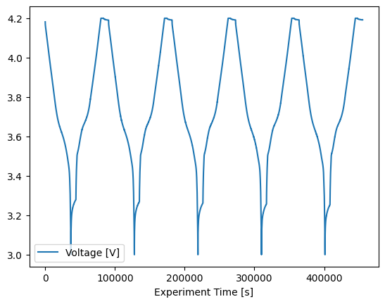
Any part of the procedure can be plotted quickly using the plot method:
cell.procedure["Sample"].experiment("Break-in Cycles").plot(
    x="Experiment Time [s]",
    y="Voltage [V]",
)
<Axes: xlabel='Experiment Time [s]'>
We can use the analysis to further analyse the data. For the 'Break-in Cycles' we will use the cycling analysis module and the functions within. These functions return Result objects, so they can be interacted with in the same ways as raw data:
from pyprobe.analysis import cycling

cycling_summary = cycling.summary(
    input_data=cell.procedure["Sample"].experiment("Break-in Cycles"),
)
print(type(cycling_summary))

print(cycling_summary.data)
<class 'pyprobe.result.Result'>
shape: (5, 8)
┌───────┬────────────┬────────────┬────────────┬────────────┬────────────┬────────────┬────────────┐
│ Cycle ┆ Capacity   ┆ Time [s]   ┆ Charge     ┆ Discharge  ┆ SOH Charge ┆ SOH        ┆ Coulombic  │
│ ---   ┆ Throughput ┆ ---        ┆ Capacity   ┆ Capacity   ┆ [%]        ┆ Discharge  ┆ Efficiency │
│ i64   ┆ [Ah]       ┆ f64        ┆ [Ah]       ┆ [Ah]       ┆ ---        ┆ [%]        ┆ ---        │
│       ┆ ---        ┆            ┆ ---        ┆ ---        ┆ f64        ┆ ---        ┆ f64        │
│       ┆ f64        ┆            ┆ f64        ┆ f64        ┆            ┆ f64        ┆            │
╞═══════╪════════════╪════════════╪════════════╪════════════╪════════════╪════════════╪════════════╡
│ 0     ┆ 0.0        ┆ 28448.2    ┆ 0.041086   ┆ 0.040937   ┆ 100.0      ┆ 100.0      ┆ null       │
│ 1     ┆ 0.082022   ┆ 119273.495 ┆ 0.041247   ┆ 0.041138   ┆ 100.393179 ┆ 100.490732 ┆ 1.001267   │
│ 2     ┆ 0.164407   ┆ 210305.197 ┆ 0.04132    ┆ 0.041241   ┆ 100.5711   ┆ 100.743512 ┆ 0.999854   │
│ 3     ┆ 0.246969   ┆ 301386.6   ┆ 0.041362   ┆ 0.041296   ┆ 100.672765 ┆ 100.876766 ┆ 0.999406   │
│ 4     ┆ 0.329627   ┆ 392471.001 ┆ 0.04139    ┆ 0.041329   ┆ 100.740624 ┆ 100.959186 ┆ 0.999212   │
└───────┴────────────┴────────────┴────────────┴────────────┴────────────┴────────────┴────────────┘
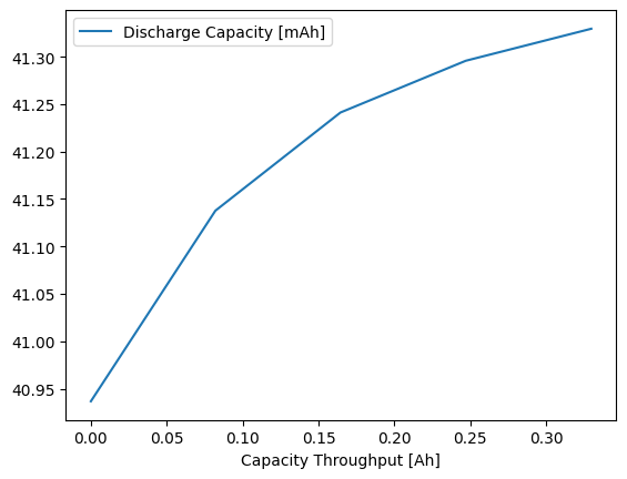
And it can be plotted as normal too:
cycling_summary.plot(x="Capacity Throughput [Ah]", y="Discharge Capacity [mAh]")
<Axes: xlabel='Capacity Throughput [Ah]'>
As the procedure that we imported without a README file does not contain experiment information, the Break-in Cycles will not work on it:
cycling_summary = cycling.summary(
    input_data=cell.procedure["Sample Quick"].experiment("Break-in Cycles"),
)
14:53:52 | ERROR | pyprobe.filters:experiment:364 - Break-in Cycles not in procedure. | Context: {}
---------------------------------------------------------------------------
ValueError                                Traceback (most recent call last)
Cell In[16], line 2
      1 cycling_summary = cycling.summary(
----> 2     input_data=cell.procedure["Sample Quick"].experiment("Break-in Cycles"),
      3 )

File ~/checkouts/readthedocs.org/user_builds/pyprobe/checkouts/stable/pyprobe/filters.py:365, in Procedure.experiment(self, *experiment_names)
    363         error_msg = f"{experiment_name} not in procedure."
    364         logger.error(error_msg)
--> 365         raise ValueError(error_msg)
    366     steps_idx.append(self.readme_dict[experiment_name]["Steps"])
    367 flattened_steps = utils.flatten_list(steps_idx)

ValueError: Break-in Cycles not in procedure.
However, all other filters will still work as expected.